SMLDS_LAB
PRG 1 : A dataset contains the prices of houses in a city. Find the 25th and 75th percentiles and calculate the interquartile range (IQR). How does the IQR help in understanding the price variability?
import numpy as np
import matplotlib.pyplot as plt
import seaborn as sns
import pandas as pd
file_path=input("Enter the Data Set : ")
#file_path="/home/ailab/GA/exp1/house_prices_india.csv"
try:
df=pd.read_csv(file_path)
print("\n~~ Dataset loaded successfully~~")
print(df.head())
if df.shape[1]>1:
print("\n available colums",list(df.columns))
column_name=input("enter the column name containing house prices:")
else:
column_name=df.columns[0]
house_prices=df[column_name].dropna().values
house_prices=house_prices[house_prices>0]
print(f"\n total no of valid house prices {len(house_prices)}")
q1=np.percentile(house_prices,25)
q3=np.percentile(house_prices,75)
print(f"\nThe 25th percentile(Q1) of hosue price is:${q1:,.2f}")
print(f"The 75th percentile (Q3) of house price is:${q3:,.2f}\n")
iqr=q3-q1
print(f"the interquartile (IQR) of house price is ${iqr:,.2f}\n")
except FileNotFoundError:
print("File not found.please check the file path")
except pd.errors.EmptyDataError:
print("File is empty or corrupted")
except Exception as e:
print(f"An error occured :{e}")
plt.figure(figsize=(10,6))
sns.boxplot(y=house_prices,color='skyblue')
plt.hlines(q1,xmin=-0.4,xmax=0.4,colors='red',linestyles='dashed',label=f'Q1(${q1:,.0f})')
plt.hlines(q3,xmin=-0.4,xmax=0.4,colors='green',linestyles='dashed',label=f'Q3(${q3:,.0f})')
plt.text(-0.45,q1,'Q1',va='center',ha='right',color='red',fontsize=12)
plt.text(-0.45,q3,'Q3',va='center',ha='right',color='green',fontsize=12)
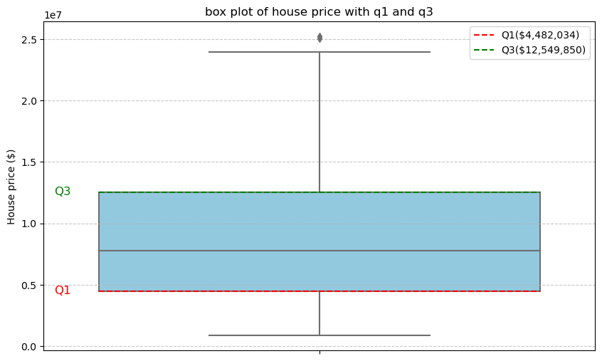
plt.title("box plot of house price with q1 and q3")
plt.ylabel("House price ($)")
plt.grid(axis='y',linestyle="--",alpha=0.7)
plt.legend()
plt.show()
plt.figure(figsize=(12,7))
sns.histplot(house_prices,kde=True,color='purple',bins=30)
plt.axvline(q1,color='red',linestyle='dashed',linewidth=2,label=f'Q1:${q1:.0f}')
plt.axvline(q3,color='green',linestyle='dashed',linewidth=2,label=f'Q3:${q3:.0f}')
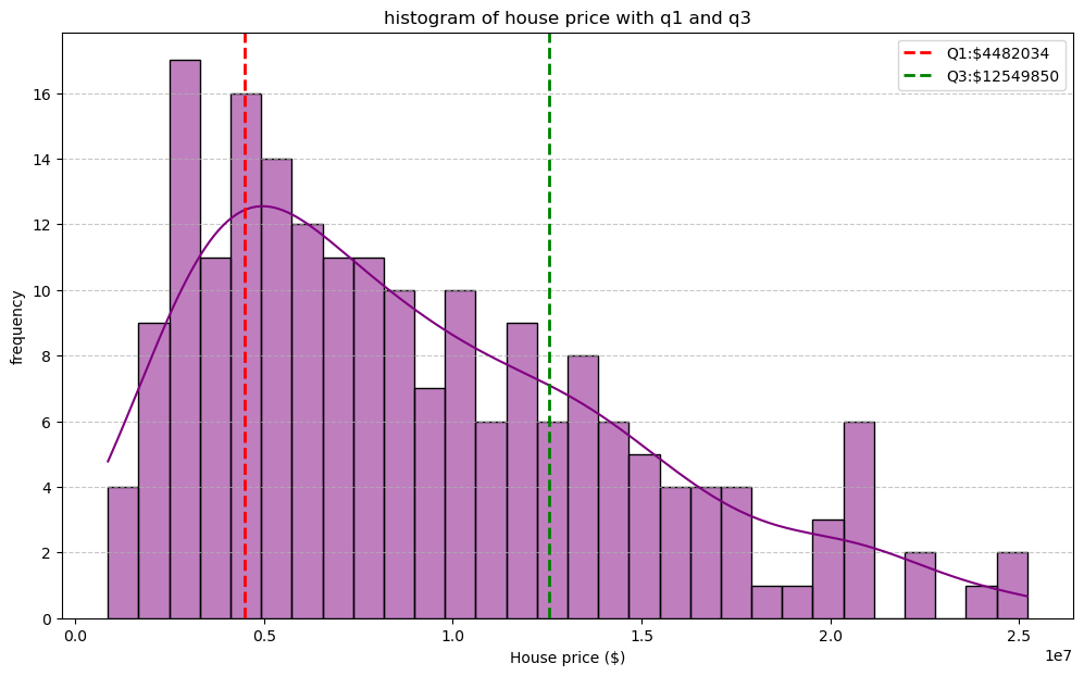
plt.title("histogram of house price with q1 and q3")
plt.xlabel("House price ($)")
plt.ylabel('frequency')
plt.legend()
plt.grid(axis='y',linestyle="--",alpha=0.7)
plt.show()
~~ Dataset loaded successfully~~
      price        availability   location   size  total_sqft  balcony
0   3069998  Under Construction  Hyderabad  1 BHK        1189        1
1  11494560       Ready To Move  Bengaluru  3 BHK        1555        0
2  13014855  Under Construction   Gurugram  3 BHK        1659        1
3   4013190  Under Construction     Nagpur  2 BHK        1037        0
4  12490569  Under Construction     Jaipur  3 BHK        1963        1

 available colums ['price', 'availability', 'location', 'size', 'total_sqft', 'balcony']
enter the column name containing house prices:price

 total no of valid house prieces 200

The 25th percentile(Q1) of hosue price is:$4,482,034.50
The 75th percentile (Q3) of house price is:$12,549,849.75

the interquartile (IQR) of house price is $8,067,815.25
Understanding price variability with IQR
The Interquartile Range (IQR) is a measure of statistical dispersion , representing the range between the upper quartile (75th percentile) and the lower quartile (25th percentile). It encompasses the central; 50% of the data. In this context,
- Robustness to Outliers:
Unlike the full range(max-min), theIQR is not influenced by extreme values providing a more stable measure of spread. - Concentration of Data:
A smaller IQR suggest that prices are tightly clustered, indicating lower variability. - Spread of Middle Values:
A larger IQR suggest more variability in typical house prices.Thus, the IQR offers a focused and robust view of variability in housing pricing